TUTORIAL 3: Dispersion mapping as an alternative to hemodynamic lag
This tutorial comprises a template data analysis script that utilizes native matlab functions as well as functions from the seeVR toolbox. If you use any part of this process or functions from this toolbox in your work please cite the following article:
Bhogal AA.,Medullary vein architecture modulates the white matter BOLD cerebrovascular reactivity signal response to CO2: observations from high-resolution T2* weighted imaging at 7T. Neuroimage 15 Dec, 2021. Vol 245, https://doi.org/10.1016/j.neuroimage.2021.118771
... and toolbox
Bhogal AA, (2021), abhogal-lab/seeVR: v1.01 (v1.01). Zenodo. https://doi.org/10.5281/zenodo.5283595
If you have suggestions for improvement, please contact me at a.bhogal@umcutrecht.nl, https://www.seevr.nl/contact-collaboration/ or feel free to start a new branch at https://github.com/abhogal-lab/seeVR
************************************************************************************************************************************
loadTimeseries: wrapper function to load nifti timeseries data using native matlab functions
loadMask: wrapper function to load nifti mask/image data using native matlab functions
meanTimeseries: calculates the average time-series signal intensity in a specific ROI
normTimeseries: normalizes time-series data to a specified baseline period
remLV: generates a mask that can be used to isolate and remove large vessel signal contributions
convHRF/convHRF2: convolves input vector (in this case PetCO2/O2) with a double-gamma HRF
scrubData: uses nuisance regressors to remove unwanted signal contributions
denoiseData: temporally de-noises data using a wavelet or moving-window based method (toolbox dependent)
smthData: perfomes gaussian smoothing operation on image/time-series data
lagCVR: calculates CVR and hemodynamic lag using a cross-correlation or lagged-GLM approach. Hemodynamic maps and optimized BOLD regressor are output/.
fitHRF2: fits a user-generated series of HRF-convolved response functions to generate dispersion and onset parameter maps
*************************************************************************************************************
MRI Data Properties
This example uses BOLD data acquired using a Philips 7 tesla MRI scanner with the
following parameters:
Scan resolution (x, y): 136 133
Scan mode: MS
Repetition time [ms]: 3000
Echo time [ms]: 25
FOV (ap,fh,rl) [mm]: 217.600 68.800 192.000
Scan Duration [sec]: 369
Slices: 43
Volumes: 120
EPI factor: 47
Slice thickness: 1.6mm
Slice gap: none
In-place resolution (x, y): 1.5mm
MRI Data Processing
Simple pre-processing of MRI data was done using FSL (https://fsl.fmrib.ox.ac.uk/fsl/fslwiki/) as follows
1) motion correction (MCFLIRT)
2) calculate mean image (FSLMATHS -Tmean)
3) brain extraction (BET f = 0.2 -m)
4) tissue segmentation on BOLD image (FAST -t 2 -n 3 -H 0.2 -I 6 -l 20.0 -g --nopve -o)
************************************************************************************************************************************
Analysis Pipeline
1) Setup options structure and load data
The seeVR functions share parameters using the 'opts' structure. In the current version this is implemented as a global variable (subect to change in the future). To get started, first initialize the global opts struct. Nifti data can be loaded using the loadTimeseries/LoadMask wrapper functions based on the native matlab nifti functions (or 'loadImageData' using provided nifti functions - see which one works for you). This function will also initialize certain variables in the opts structure including opts.TR (repetition time). opts.dyn (number of volumes), opts.voxelsize (resolution), and opts.info ( if using loadTimeseries then opts.headers is initialized and used by saveImageData to save timeseries, parameter maps and masks in opts.headers.ts/map/mask).
*If you use your own functions to load your imaging data, ensure that you also fill the above fields in the opts structure to ensure maintained functionality (especially opts.TR). If functions throw errors, it is usually because a necessary option is not specified before the function call.
clear all
clear global all
close all
% initialize the opts structure (!)
global opts
opts.verbose = 0;
% Set the location for the MRI data
dir = 'UPDATE TO YOUR OWN PATH WHERE DATA IS SAVED\';
cd(dir)
% Load motion corrected data
filename = 'BOLD_masked_mcf.nii.gz';
[BOLD,INFO] = loadTimeseries(dir, filename);
% Load GM segmentation
file = 'BOLD_mean_brain_seg_0.nii.gz';
[GMmask,INFOmask] = loadMask(dir, file);
% Load WM segmentation
file = 'BOLD_mean_brain_seg_1.nii.gz';
[WMmask,~] = loadMask(dir, file);
% Load CSF segmentation
file = 'BOLD_mean_brain_seg_2.nii.gz';
[CSFmask,~] = loadMask(dir, file);
% Load brain mask
file = 'BOLD_mean_brain_mask.nii.gz';
[WBmask,~] = loadMask(dir, file);
2) Setup directories for saving output
Pay special attention to the savedir, resultsdir and figdir as you can use these to organize the various script outputs.
% specify the root directory to save results
opts.savedir = dir;
% specify a sub directory to save parameter maps - this
% directory can be changed for multiple runs etc.
if ispc
opts.resultsdir = [dir,'RESULTS\']; mkdir(opts.resultsdir);
else
opts.resultsdir = [dir,'RESULTS/']; mkdir(opts.resultsdir);
end
% specify a sub directory to save certain figures - this
% directory can be changed for multiple runs etc.
if ispc
opts.figdir = [dir,'FIGURES\']; mkdir(opts.figdir);
else
opts.figdir = [dir,'FIGURES/']; mkdir(opts.figdir);
end
3) Take a quick look at the data
Use the 'meanTimeseries' function with any mask to look at the ROI timeseries. To see the differences between GM, WM and whole-brain timeseries, use the 'normTimeseries' function before plotting using the 'meanTimeseries' function. As you can see in the figure, there are three signal peaks corresponding to three hypercapnic periods delivered using a RespirAct system.
% Normalized BOLD data to 20 volumes in baseline period
% if no index is provided, baseline can be selected manually
nBOLD = normTimeseries(BOLD, WBmask, [5 25]);
TS1 = meanTimeseries(nBOLD, GMmask);
%establish new xdata vector for plotting
xdata = opts.TR:opts.TR:opts.TR*size(nBOLD,4);
% Plot GM timeseries
figure;
plot(xdata, TS1, 'k'); title('time-series data');
ylabel('absolute signal'); xlabel('time (s)'); xlim([0 xdata(end)])
% Overlay WM timeseries
hold on
TS2 = meanTimeseries(nBOLD, WMmask);
plot(xdata, TS2, 'm');
set(gcf, 'Units', 'pixels', 'Position', [200, 500, 600, 160]);
legend('GM','WM')
hold off

clear TS1 TS2 nBOLD
4) Load end-tidal gas traces
For simplicity I have already aligned the gas traces. Simply load them from the example dataset. If loading your own data, you can use the 'resampletoTR' function to interpolate breathing data to the same temporal resolution as your MRI data. For alignment, use the trAlign function (see tutorial 1).
cd(dir)
load('traces.mat')
5) Regress out motion parameters
To regress out motion parameters (or whatever other nuisance data you can think of), use the 'scrubData' function. This function accepts an array or nuisance regressors and data regressors. For the data probe we will use the end-tidal CO2 trace. You can also consider to first convolve the CO2 trace with an HRF using the ' convHRF' or ' convEXP' functions (see manual). Sometimes motion parameters are correlated with your task - this can be due to real motion (i.e. head movement during breath-hold or hyperventilation at high CO2) or effects related to changing signal intensity due to increased CBF that are confused as motion by the realignment algorithm. If including such regressors you risk removing signals of interest. To filter these you can use the ' filtRegressor' function.
cd(dir) % Go to our data directory
%mpfilename = 'BOLD_mcf.par'; % Find MCFLIRT motion parameter file
mpfilename = 'BOLD_masked_mcf.par'; % Find MCFLIRT motion parameter file
nuisance = load(mpfilename); % Load nuisance regressors (translation, rotation etc.)
% Calculate motion derivatives
dtnuisance = gradient(nuisance); % temporal derivative
sqnuisance = nuisance.*nuisance; % square of motion
motion = [nuisance dtnuisance sqnuisance];
% Demean/rescale regressors
for ii=1:(size(motion,2)); motion(:,ii) = demeanData(rescale(motion(:,ii))); end
% Filter regressors
reference = meanTimeseries(BOLD,GMmask);
opts.motioncorr = 0.3; % correlation (r) threshold
[keep, leave] = filtRegressor(motion, reference, opts);
% Attempt to clean all voxels contained in the WB mask using nuisance
% regressors. In this example, there are not many motion related artifacts.
opts.disp = [1 3 6 9]; %dispersion
[~,~,HRF_probe_CO2] = convHRF(CO2trace, opts);
%regression
% add a linear term to acount for signal drift
% Data scrubbing
[cleanData] = scrubData(BOLD,WBmask, keep, [HRF_probe_CO2], opts);


% You can also consider to include the nuisance probes with high
% correlation to the reference signal as data probes or a linear term
%L = rescale(LegendreN(1,xdata));
%[cleanData] = scrubData(BOLD,WBmask, [L' keep], [HRF_probe_CO2' leave], opts);
% plot results
figure;
plot(xdata, meanTimeseries(BOLD,WBmask), 'k');
hold on
plot(xdata, meanTimeseries(cleanData,WBmask), 'm');
xlabel('time (s)'); ylabel('absolute signal');
title('whole-brain average signal')
legend('before cleanup', 'after cleanup');
set(gcf, 'Units', 'pixels', 'Position', [200, 500, 600, 160]);
xlim([0 xdata(end)]); hold off

6) Removing contributions using a large vessel mask
CVR data can often be weighted by contributions from large vessels that may overshadow signals of interest. Particulary, for very high resolution acquisitions at high field strength. We can modify the whole brain mask to exclude CSF and large vessel contributions using the 'remLV' function ('remove large vessels'). This can be done by specifying the percentile threshold from which to remove voxels, or if the appropriate toolbox is not available, a manual threshold value.
% Supply necessary options
% Define the cutoff percentile (higher values are removed; default = 98);
opts.LVpercentile = 98.5;
% If the stats toolbox is not present, then a manual threshold must
% be applied. This can vary depending on the data (i.e. trial and error).
[mWBmask] = remLV(cleanData,WBmask,opts);
%plot results
figure;
z = 30;
subplot(1,3,1)
imagesc(imrotate(mean(BOLD(:,:,z,:),4),90));
title('mean image', 'Color', 'w'); colormap(gray); cleanPlot;
subplot(1,3,2)
imagesc(imrotate(WBmask(:,:,z),90));
title('original mask', 'Color', 'w'); cleanPlot;
subplot(1,3,3)
imagesc(imrotate(mWBmask(:,:,z),90));
title('modified mask', 'Color', 'w'); cleanPlot;
set(gcf, 'Units', 'pixels', 'Position', [200, 500, 600, 160]);

7) Temporally de-noise data
To remove spikes from motion or high frequency noise these try the 'denoiseData' function. When the wavelet toolbox is available, this function uses a wavelet-based approach. Otherwise a more simple gaussian approach is applied however this can result in a temporal shift. Low-pass filtering is another option - this can be done via output from the 'glmCVRidx' function (see manual).
%de-noise
denBOLD = denoiseData(cleanData, WBmask, opts);
% Check results
figure; hold on;
plot(xdata, meanTimeseries(cleanData,GMmask), 'k', 'LineWidth',2);
plot(xdata, meanTimeseries(denBOLD,GMmask), 'c', 'LineWidth',2);
title('noise removal');
ylabel('absolute signal'); xlabel('time (s)'); legend('original', 'de-noised')
set(gcf, 'Units', 'pixels', 'Position', [200, 500, 600, 160]); xlim([0 xdata(end)])
hold off

8) Smooth and normalize data
Here we will use some of the default parameters from the 'smthData' function. This means we do not need to pass any parameters in the opts struct (defaults are: opts.FWHM = 4mm, opts.filtWidth = 5)
% 3d Gaussian smoothing
opts.spatialdim = 3; %default = 2
opts.FWHM = 3;
sBOLD = smthData(denBOLD, mWBmask, opts);
% Normalize data to first 15 baseline images
nBOLD = normTimeseries(sBOLD,mWBmask,[5 25]);
clear sBOLD denBOLD
9) Dispersion Mapping
Hemodynamic lag calculations (see tutorial #1) provides information on possible blood flow delays. Generally, the lag is expressed in seconds or TR but is not always reflective of true temporal effects. Often, correlations can be weighed by the time-to-peak of the BOLD signal response. This can be seen when comparing white matter and grey matter time courses. The white matter signal rises more slowly and this leads to longer delays. However, the onset of the white matter response is often close to that of the GM. This effect is can be termed 'signal dispersion', and may be related to draining vein effects. See: https://doi.org/10.1016/j.neuroimage.2021.118771 and https://pubmed.ncbi.nlm.nih.gov/26126862/.
The 'fitHRF2' function can be used to produce 'HRF maps' that represent voxel-wise information related to signal onset and dispersion. This function first produces a 'look-up' table of possible user defined responses generated using the opts.onset and opts.disp parameters.
%First we will generate an initial probe using the lagCVR function.
%This probe will represent the 'fastest' intrinsic responses to the
%vasoactive stimulus and will already show inherent changes that
% occur as the CO2 bolus moves from the lungs to the brain and then
% the cerebral draining veins. To save processing time, mapping options for
% lagCVR can be turned off:
opts.corr_model = 0; %set to 0 for optimized probe output only
opts.glm_model = 0; %set to 0 for optimized probe output only
opts.cvr_maps = 0; %set to 0 for optimized probe output only
% Factor by which to temporally interpolate data. Better for picking up
% lags between TR. Higher value means longer processing time and more RAM
% used (so be careful)
opts.interp_factor = 2; %default is 4
% The correlation threshold is an important parameter for generating the
% optimized regressor. For noisy data, a too low value will throw an error.
% Ideally this should be set as high as possible, but may need some trial
% and error.
opts.corrthresh = 0.7; %default is 0.7
% Thresholds for refinening optimized regressors. If you make this range too large
% it smears out your regressor and lag resolution is lost. When using a CO2
% probe, the initial 'bulk' alignment becomes important here as well. A bad
% alignment will mean this range is also maybe not appropriate or should be
% widened for best results. (ASSUMING TR ~1s!, careful).
opts.lowerlagthresh = -2; %default is -3
opts.upperlagthresh = 2; %default is 3
% Lag thresholds (in units of TR) for lag map creation. Since we are looking at a healthy
% brain, this can be limited to between 20-60TRs. For impariment you can consider
% to raise the opper threshold to between 60-90TRs (ASSUMING TR ~1s!, careful).
opts.lowlag = -3; %setup lower lag limit; negative for misalignment and noisy correlation
opts.highlag = 25; %setups upper lag limit; allow for long lags associated with pathology
% For creating the optimized BOLD regressor, we will only use GM voxels for
% maximum CO2 sensitivity. We will also remove large vessel contributions.
mGMmask = GMmask.*mWBmask;
%remove CSF from analysis
mCSFmask = CSFmask -1; mCSFmask = abs(mCSFmask);
mask = mCSFmask.*mWBmask;
% Perform hemodyamic analysis
% The lagCVR function saves all maps and also returns them in a struct for
% further analysis. It also returns the optimized probe when applicable.
% uncomment this to run your own analysis
%*********************************************%
%[newprobe, maps] = lagCVR(mGMmask, mask, nBOLD, PetCO2, [], opts);
%*********************************************%
% I have provided the analyzed lag/CVR maps and optimized regressor
% comment out for your own analysis
cd(dir)
load('final_probe.mat')
% The advantage of using the global opts struct is that the variables used
% for a particular processing run (including all defaults set within
% functions themselves) can be saved to compare between runs.
save([opts.resultsdir,'processing_options.mat'], 'opts');
Fitting Dispersion
Depending on the nature of the data, convolution with the exponential or double-gamma functions can lead to varying results. Using the optimized probe (newprobe), it is helpful to first determine a range of suitable functions using the convHRF2 or convEXP2 functions. **NOTE this analysis is highly sensitive to SNR so results may vary when using your own data.
% look at onset only
opts.verbose = 1;
opts.onset = 1:1:12;
opts.disp = 1;
[b,c] = convHRF2(newprobe,opts);

set(gcf, 'Units', 'pixels', 'Position', [200, 500, 600, 160]);
% look at dispersion only
opts.onset = 1;
opts.disp = 1:2:120;
[b,c] = convHRF2(newprobe,opts);

set(gcf, 'Units', 'pixels', 'Position', [200, 500, 600, 160]);
% take some time to tune these parameters before running fitHRF2
% Generate HRF maps; **this can take quite a while depending on how you
% setup the HRF functions. The more options you supply (via onset,disp params),
% the longer it takes. Start with only a few! *NOTE: parameters should be set before each run.
% Look at combination
opts.onset = 1:1:12;
opts.disp = 1:2:120;
set(gcf, 'Units', 'pixels', 'Position', [200, 500, 600, 160]);
[b,c] = convHRF2(newprobe,opts);

% Once you are satisfied with the model functions run fitHRF with the
% appropriate options (.onset and .disp)
% uncomment this to run your own analysis
%*********************************************%
%[HRFmaps] = fitHRF2(WMmask,nBOLD,newprobe,opts); %fit dispersion
%*********************************************%
% This can take quite some time. For the sake of this tutorial, I have provided the processed maps that can be loaded
% comment out for your own analysis
cd(dir)
load('HRF_maps.mat')
HRF_maps = maps;
load('lagCVR_maps.mat')
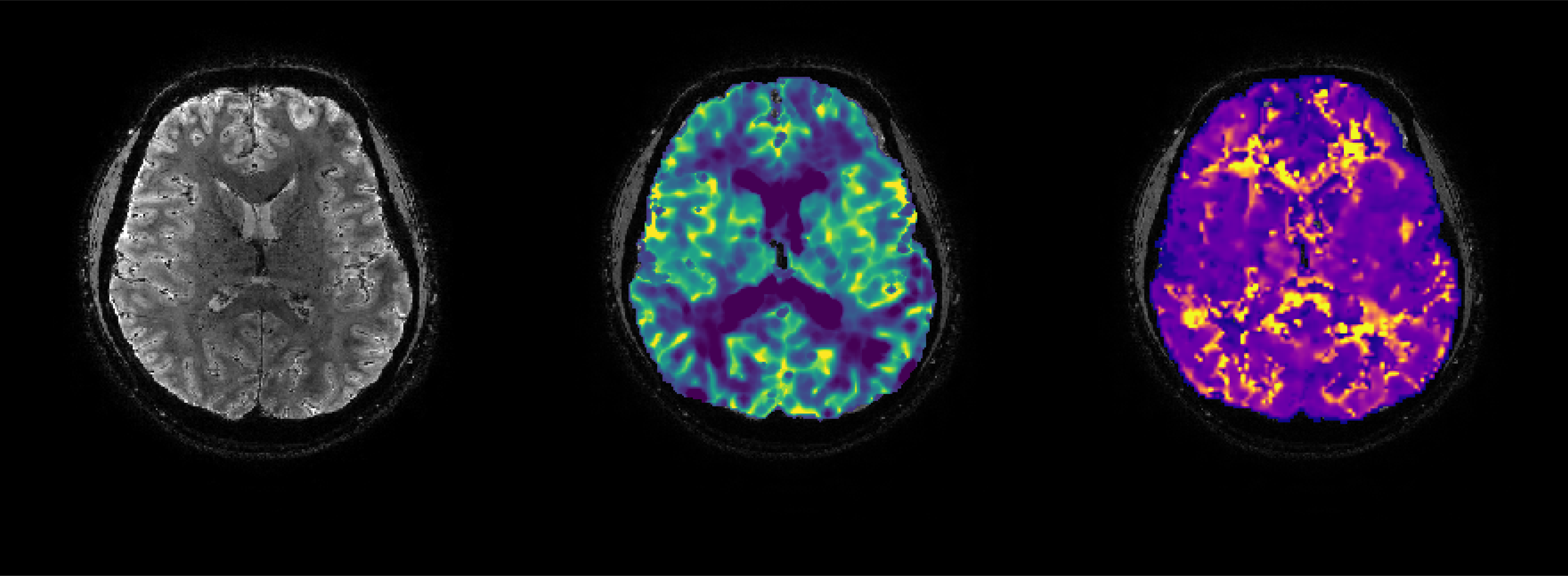
10) Plot results
% Plot lag and dispersion maps
lag_xcorr = maps.XCORR.lag_opti; lag_xcorr(lag_xcorr == 0) = NaN;
cvr_xcorr = maps.XCORR.CVR.bCVR; cvr_xcorr(cvr_xcorr == 0) = NaN;
ccvr_xcorr = maps.XCORR.CVR.cCVR; ccvr_xcorr(ccvr_xcorr == 0) = NaN;
lag_glm = maps.GLM.optiReg_lags; lag_glm(lag_glm == 0) = NaN;
cvr_glm = maps.GLM.CVR.optiReg_cCVR; cvr_glm(cvr_glm == 0) = NaN;
dispersion = HRF_maps.disp; dispersion(dispersion == 0) = NaN;
onset = HRF_maps.onset; onset(onset == 0) = NaN;
figure;
step = 5;
z=10;
scl = [0 0.5];
scllag = [0 70];
sclr = [-1 1];
r2 = [0 1];
scldisp = [0 60];
sclons = [0 10];
for ii=0:step-1
% BOLD
subplot(5,5,ii+1)
imagesc(imrotate(BOLD(:,:,z + ii*step,1),90));
colormap(gray)
freezeColors;
cleanPlot; if ii == 0; ylabel('BOLD', 'color', 'w'); end
% Lags cross-correlation
subplot(5,5,ii+1+step)
imagesc(imrotate(lag_xcorr(:,:,z + ii*step),90), scllag);
colormap(parula)
freezeColors;
cleanPlot; if ii == 0; ylabel('lags xcorr', 'color', 'w');
xlabel('lags: 0 to 70s', 'color', 'w'); end
% Lags shifted regressor GLM
subplot(5,5,(ii+1+2*step))
imagesc(imrotate(lag_glm(:,:,z + ii*step),90), scllag);
colormap(parula)
freezeColors;
cleanPlot; if ii == 0; ylabel('lags glm', 'color', 'w');
xlabel('lags: 0 to 70s', 'color', 'w'); end
subplot(5,5,(ii+1+3*step))
imagesc(imrotate(dispersion(:,:,z + ii*step),90), scldisp);
colormap(parula)
freezeColors;
cleanPlot; if ii == 0; ylabel('dispersion', 'color', 'w');
xlabel('dispersion: 0 to 60', 'color', 'w'); end
subplot(5,5,(ii+1+4*step))
imagesc(imrotate(onset(:,:,z + ii*step),90), sclons);
colormap(inferno)
freezeColors;
cleanPlot; if ii == 0; ylabel('onset', 'color', 'w');
xlabel('onset: 0 to 12', 'color', 'w'); end
end
set(gcf, 'Units', 'pixels', 'Position', [10, 100, 1000, 800]);

% plot CVR
figure;
for ii=0:step-1
% BOLD
subplot(4,5,ii+1)
imagesc(imrotate(BOLD(:,:,z + ii*step,1),90));
colormap(gray)
freezeColors;
cleanPlot; if ii == 0; ylabel('BOLD', 'color', 'w'); end
% bCVR
subplot(4,5,ii+1+step)
imagesc(imrotate(cvr_xcorr(:,:,z + ii*step),90), scl);
colormap(viridis)
freezeColors;
cleanPlot; if ii == 0; ylabel('base cvr', 'color', 'w');
xlabel('cvr: 0 to 0.50 %/mmHg', 'color', 'w'); end
% cCVR
subplot(4,5,(ii+1+2*step))
imagesc(imrotate(ccvr_xcorr(:,:,z + ii*step),90), scl);
colormap(viridis)
freezeColors;
cleanPlot; if ii == 0; ylabel('lag corrected cvr', 'color', 'w');
xlabel('cvr: 0 to 0.50 %/mmHg', 'color', 'w'); end
% cvr_glm
subplot(4,5,(ii+1+3*step))
imagesc(imrotate(cvr_glm(:,:,z + ii*step),90), scl);
colormap(viridis)
freezeColors;
cleanPlot; if ii == 0; ylabel('lag corrected cvr (glm)', 'color', 'w');
xlabel('cvr: 0 to 0.50 %/mmHg', 'color', 'w'); end
end
set(gcf, 'Units', 'pixels', 'Position', [10, 100, 1000, 640]);
